Weather Variables
This page describes all the variables that are available through the Forecast API (more information on the product page and in the technical documentation) and Dataset API (more information on the product page and in the technical documentation)
This document gives a detailed overview over all weather variables. In case of time intervals, the time indicates the end of the time interval. The values are thus backward in time sums, averages, maxima or minima. Assuming e.g. 3 hour time resolution, the precipitation value indicated at 10:00 is the precipitation amount that fell between 7:01 and 10:00. This backward in time convention has its origins in observational data, where at any given point in time you can see what was observed in the past up to the current time.
Air Quality Variables
Air Quality Index
The air quality index (dimensionless) indicates how clean or polluted the air is. Surface ozone, particulate matter, carbon monoxide, sulfur dioxide and nitrogen oxides are evaluated as pollution. A high index (>100) indicates a polluted air, combined with possible health hazards. Depending on how sensitive individuals react, the dangers can vary.
| Air quality index | Air pollution | Health implications |
|---|---|---|
| 0 - 50 | Excellent | No health implications |
| 51 - 100 | Good | Few hypersensitive individuals should reduce outdoor exercise |
| 101 - 150 | Lightly polluted | Slight irritations may occur, individuals with breathing or heart problems should reduce outdoor exercise |
| 151 - 200 | Moderately polluted | Some irritations may occur, individuals with breathing or heart problems should reduce outdoor exercise |
| 201 - 300 | Heavily polluted | Healthy people will be noticeably affected. People with breathing or heart problems will experience reduced endurance in activities. These individuals and elders should remain indoors and restrict activities |
| 300+ | Severely polluted | Healthy people will experience reduced endurance in activities. There may be strong irritations and symptoms and may trigger other illnesses. Elders and the sick should remain indoors and avoid exercise. Healthy individuals should avoid outdoor activities. |
- This variable can be found in the following package: Air Quality
CAQI
The Common Air Quality Index (CAQI) is an air quality index used in Europe since 2006.
The CAQI is a number on a scale from 1 to 100, where a low value means good air quality and a high value means bad air quality. The index is defined in both hourly and daily versions, and separately near roads (a "roadside" or "traffic" index) or away from roads (a "background" index). meteoblue is showing the background index because weather models can not reproduce small-scale difference along the roads. Therefore, measurements along roads will show higher values.
Some of the key pollutant densities in μg/m for the hourly background index, the corresponding sub-indices, and five CAQI ranges and verbal descriptions are as follows.
| Qualitative name | Index or sub-index | Pollutant (hourly) density in μg/m3 | |||
|---|---|---|---|---|---|
| NO2 | PM10 | O3 | PM2,5 | ||
| Very low | 0 - 25 | 0 - 50 | 0 - 25 | 0 - 60 | 0 - 15 |
| Low | 25 - 50 | 50 - 100 | 25 - 50 | 60 - 120 | 15 - 30 |
| Medium | 50 - 75 | 100 - 200 | 50 - 90 | 120 - 180 | 30 - 55 |
| High | 75 - 100 | 200 - 400 | 90 - 180 | 180 - 240 | 55 - 110 |
| Very high | > 100 | > 400 | > 180 | > 240 | > 110 |
- The variables can be found in the following package: Air Quality
Ozone Concentration
Ozone (O) is a trace gas, which resides mainly in the stratosphere (90%) with a peak at an altitude of 25 km (ozone layer), where it absorbs the harmful solar UV radiation. The other 10% resides in the troposphere. Near the Earth's surface, ozone is a harmful pollutant, that can cause damage to the lung and other organs. Anthropogenic ozone pollution in the lower troposphere is caused mainly in urban areas where ozone is a result of photochemical reactions of nitrogen oxides and hydrogen carbons. The tropospheric ozone is unequally distributed and concentrations vary.
The ozone concentration is expressed in microgram per cubic meter (μg/m) as well as in mole fraction (parts per billion, ppb) or Dobson Units (DU), which indicates the total-column ozone. Dobson Units show the theoretical thickness (in units of 10 µm) of the layer the gas would form, if it is set under standard temperature (0°C) and pressure (1013.25 hPa). For instance, 300 DU of ozone would form a layer 3 mm thick.
Ozone can be found at the surface but also very high up in the atmosphere. The upper air ozone in the stratosphere protects us from the very harmful UV-C and UV-B radiation. The lack of this stratospheric ozone is known as the ozone hole which can lead to severe health risks especially in the Southern hemisphere. For these reasons, a high ozone concentration in the stratosphere is positive, but near the surface it can be detrimental to human health. The meteoblue maps show the ozone concentration at the surface. Ozone in the air we breathe can harm our health, especially on hot sunny days when ozone can reach high concentrations. Even relatively low levels of ozone can cause health effects. Most at risk from breathing air containing ozone are people with asthma, children, older adults, and people who are active outdoors, especially outdoor workers.
Ozone can:
- Make it more difficult to breathe deeply and vigorously
- Cause shortness of breath, and pain when taking a deep breath
- Cause coughing and sore or scratchy throat
- Inflame and damage the airways
- Aggravate lung diseases such as asthma, emphysema, and chronic bronchitis
- Increase the frequency of asthma attacks
- Make the lungs more susceptible to infection
- Continue to damage the lungs even when the symptoms have disappeared
- Cause chronic obstructive pulmonary disease (COPD)
- This variable can be found in the following package: Air Quality
Pollen
Currently, we provide forecasts of Birch, Grass and Olive pollen. Birch pollen is one of the most common airborne allergens during springtime, or later in the year in higher latitudes. As the trees bloom, they release tiny grains of pollen that are scattered by the wind. A single birch tree can produce up to five million pollen grains. Pollen is dispersed by air currents and can be transported over large distances. We thus show the pollen forecast overlayed with the 10 m wind speed.
Grass pollen are the primary trigger of pollen allergies during the summer months. It causes some of the most severe and difficult-to-treat symptoms. In humid climates, the grass pollen season can be several months, in drier climates the grass pollen season is significantly shorter, as are the birch and olive pollen season.
Precipitation can clean the air from pollen, but if it is associated with thunderstorms, the strong winds initially increase the pollen concentration.
- The variables can be found in the following package: Air Quality
Desert Dust Concentration
The desert dust concentration indicates how much desert dust is contained in the air and it is given in six classes:
| Colour | Concentration |
|---|---|
| Green | < 40 μg/m³ |
| Light green | < 80 μg/m³ |
| Yellow | < 160 μg/m³ |
| Light orange | < 450 μg/m³ |
| Dark orange | < 1000 μg/m³ |
| Red | > 1000 μg/m³ |
At high concentration, desert dust can be perceived as a veil. The individual particles appear as condensation nuclei and lead to cloud formation.
- This variable can be found in the following package: Air Quality
PM10 and PM2.5
Atmospheric particulate matter (PM) are microscopic solid or liquid matter suspended in the air. Sources of particulate matter can be natural or anthropogenic.
Of greatest concern to public health are the particles small enough to be inhaled into the deepest parts of the lung. These particles are less than 10 microns in diameter (approximately 1/7th the thickness of the a human hair) and are known as PM10. They are among the most harmful of all air pollutants. Health problems begin as the body reacts to these foreign particles. PM10 can increase the number and severity of asthma attacks, cause or aggravate bronchitis and other lung diseases, and reduce the body's ability to fight infections.
Although particulate matter can cause health problems for everyone, certain people (the elderly, exercising adults, and those suffering from asthma or bronchitis) are especially vulnerable to PM10.
PM10 is a mixture of materials that can include smoke, soot, dust, salt, acids, and metals. Particulate matter also forms when gases emitted from motor vehicles and industry undergo chemical reactions in the atmosphere. PM10 is visible by eye as the haze that we think of as smog.
PM10 includes fine particulate matter known as PM2.5, which are fine particles with a diameter of 2.5 μm or less. The biggest impact of particulate air pollution on public health is understood to be from long-term exposure to PM2.5, which increases the age-specific mortality risk, particularly from cardiovascular causes.
- This variable can be found in the following package: Air Quality
SO (Sulfur Dioxide)
Sulfur dioxide is a gas, which is invisible and has a nasty, sharp smell. It reacts easily with other substances to form harmful compounds, such as sulfuric acid, sulfurous acid and sulfate particles. Short-term exposures to SO can harm the human respiratory system and make breathing difficult. Children, the elderly, and those who suffer from asthma are particularly sensitive to effects of SO. SO and other sulfur oxides can contribute to acid rain which can harm sensitive ecosystems.
About 99% of the sulfur dioxide in air comes from human sources. The main source of sulfur dioxide in the air is industrial activity that processes materials that contain sulfur, e.g. the generation of electricity from coal, oil or gas that contains sulfur. Some mineral ores also contain sulfur, and sulfur dioxide is released when they are processed. In addition, industrial activities that burn fossil fuels containing sulfur can be important sources of sulfur dioxide.
Sulfur dioxide is also present in motor vehicle emissions, as the result of fuel combustion.
Source: https://www.dcceew.gov.au/environment/protection/npi/substances/fact-sheets/sulfur-dioxide
- This variable can be found in the following package: Air Quality
CO (Carbon Monoxide)
Carbon monoxide (CO) is a colorless, odorless, and tasteless gas that is slightly less dense than air. It is toxic to humans when encountered in concentrations above about 35 ppm, although it is also produced in normal animal metabolism in low quantities, and is thought to have some normal biological functions. In the atmosphere, it is spatially variable and short lived, having a role in the formation of ground-level ozone.
Carbon monoxide is present in small amounts in the atmosphere, chiefly as a product of volcanic activity but also from natural and man-made fires (such as forest and bushfires, burning of crop residues, and sugarcane fire-cleaning). The burning of fossil fuels also contributes to carbon monoxide production. Carbon monoxide occurs dissolved in molten volcanic rock at high pressures in the Earth's mantle. Because natural sources of carbon monoxide are so variable from year to year, it is extremely difficult to accurately measure natural emissions of the gas.
Carbon monoxide is a short-lived greenhouse gas and also has an indirect radiative forcing effect by elevating concentrations of methane and tropospheric ozone through chemical reactions with other atmospheric constituents (e.g., the hydroxyl radical, OH.) that would otherwise destroy them. Through natural processes in the atmosphere, it is eventually oxidized to carbon dioxide. Carbon monoxide is both short-lived in the atmosphere (on average about two months) and spatially variable in concentration.
- This variable can be found in the following package: Air Quality
NO (Nitrogen Dioxide)
Nitrogen dioxide is one of several nitrogen oxides. NO is an intermediate in the industrial synthesis of nitric acid, millions of tons of which are produced each year. At higher temperatures it is a reddish-brown gas that has a characteristic sharp, biting odor and is a prominent air pollutant.
The major source of nitrogen dioxide is the burning of fossil fuels: coal, oil and gas. Most of the nitrogen dioxide in cities comes from motor vehicle exhaust. NO is also introduced into the environment by natural causes, including entry from the stratosphere, bacterial respiration, volcanos, and lightning. These sources make NO a trace gas in the atmosphere of Earth, where it plays a role in absorbing sunlight and regulating the chemistry of the troposphere, especially in determining ozone concentrations.
Nitrogen dioxide is an important air pollutant because it contributes to the formation of ozone, which can have significant impacts on human health.
NO can:
- inflame the lining of the lungs, and it can reduce immunity to lung infections
- cause problems such as wheezing, coughing, colds, flu and bronchitis
- This variable can be found in the following package: Air Quality
Aerosol Optical Depth
The optical depth is a measure of how well electromagnetic waves can pass through a medium. Therefore, the aerosol optical depth is the measure for the reduction of light transmission caused by atmospheric aerosols. It describes the total light extinction in the vertical atmospheric column, which depends on the light's wavelength and the amount of atmospheric aerosols. The greater the value of optical depth, the greater the aerosol concentration. Sources of aerosol can be diverse: wild fire, desert dust or anthropogenic air pollution. The aerosol optical depth is dimensionless.
- This variable can be found in the following package: Air Quality
Visibility
Visibility is the distance (in metres (m)) at which an object can be clearly seen. Note that visibility is extremely difficult to forecast especially if visibility is reduced to less than 3000 m.
The indicated visibility applies to the point in time that is specified.
Cloud Variables
Cloud Cover
Cloud cover is expressed in percent (%). Zero means that there is no visible cloud in the sky. Fifty percent is equivalent to half of the sky being covered with clouds. Hundred percent cloud cover means no clear sky is visible. Cloud cover can be divided into:
- Low cloud cover: 0 - 4 km/ below an altitude of 640 hPa (5 km at equator)
- Mid cloud cover: 4 - 8 km/ between an altitude of 640 and 350 hPa (10 km at equator)
- High cloud cover: 8 - 15 km/ between an altitude of 350 and 150 hPa (18 km at equator) Note that high clouds are thin ice clouds which, even when reaching 100%, might be almost invisible in some cases
The indicated cloud cover applies to the point in time that is specified.
- This variable can be found in the following packages: Clouds, Profile Series, Multimodel, Trend, Trend Pro, Seasonal Anomalies Forecast and the History API
Cloud Ice
Total atmospheric column frozen water content of all clouds, excluding precipitation. It's unit is gram (g).
The indicated cloud ice applies to the point in time that is specified.
- This variable can be found in the following package: Air
Cloud Water
Total atmospheric column liquid water content of all clouds, excluding precipitation. It's unit is gram (g).
The indicated cloud ice applies to the point in time that is specified.
- This variable can be found in the following package: Air
Humidity
Dew Point Temperature
The dew point is the point at which dew starts to form on solid surfaces (that is for example the drops on grass that appear early in the morning). By definition it is the air temperature (°C) at which a specific volume of air (that has a constant pressure) condenses water vapour into liquid water at the same rate as it evaporates. This also means that the vapour pressure is equal to the saturation vapour pressure. If the relative humidity is 100%, the dew point temperature is the same as the air temperature. Thus the air is saturated. If the temperature decreases, but the amount of water vapour stays constant, water will start to condensate. This condensed water is called dew as soon as it forms on a solid surface. It is expressed in degrees Celsius (°C) as well as in degrees Fahrenheit (°F).
The indicated dew point temperature applies to the point in time that is specified.
- This variable can be found in the following packages: Agro, Trend Pro, Seasonal Anomalies Forecast and the History API
Relative Humidity
Relative humidity indicates how saturated the air is with moisture (expressed in percent (%)). If relative humidity approaches 100%, then clouds / fog begin to form. Note that relative humidity is strongly dependent on air temperature, keeping the amount of water equal, relative humidity decreases with increasing temperature.
The indicated relative humidity applies to the point in time that is specified.
- This variable can be found in the following packages: Basic, Sigma Level, Profile Series, Single Variable Multimodel, Trend, Trend Pro and the History API
Vapour Pressure Deficit
Vapour pressure deficit (VPD) corresponds to the difference between the amount of moisture in the air and how much moisture the air can still absorb at a certain temperature until it is saturated. It is given in hPa. The vapour pressure deficit is strongly dependent on temperature, but hardly on pressure.
The indicated vapour pressure deficit applies to the point in time that is specified.
- This variable is only available with Dataset API
Vapour Pressure Saturation
The saturation vapour pressure is defined as the pressure at which the gaseous state is in equilibrium with the liquid or solid state. The saturation vapour pressure depends on the temperature.
The indicated vapour pressure saturation applies to the point in time that is specified.
- This variable is only available with Dataset API
Evapotranspiration
The indicated evapotranspiration is the sum over the preceeding time period.
- This variable can be found in the following packages: Agro, Trend Pro, Seasonal Anomalies Forecast and the History API
Potential Evapotranspiration
Potential evapotranspiration is a theoretical value and explains how much water would evaporate from a water surface. It is often not realistic, for example, the value of potential evapotranspiration in the Sahara is very large, but actually there is no water to evaporate. Potential evapotranspiration is expressed in millimetre (mm).
The indicated potential evapotranspiration is the sum over the preceeding time period.
- This variable can be found in the following package: Agro
Total Evapotranspiration
Sum of evaporation (soils, lakes, seas) and transpiration (plants). It assumes a non irrigated surface, thus only the naturally available water. For irrigated crops this value will be too low and we recommend using the Reference Evapotranspiration instead. Total evapotranspiration is described in millimetre (mm).
The indicated total evapotranspiration is the sum over the preceeding time period.
Reference Evapotranspiration (Eto)
The so-called reference crop evapotranspiration or reference evapotranspiration, denoted as ETo. The reference surface is a hypothetical grass reference crop with an assumed crop height of 0.12 m, a fixed surface resistance of 70 sm and an albedo of 0.23. The reference surface closely resembles an extensive surface of green, well-watered grass of uniform height, actively growing and completely shading the ground. The fixed surface resistance of 70 sm implies a moderately dry soil surface resulting from about a weekly irrigation frequency. As a result of an Expert Consultation held in May 1990, the FAO Penman- Monteith method is now recommended as the sole standard method for the definition and computation of the reference evapotranspiration.
The indicated reference evapotranspiration is the sum over the preceeding time period.
- This variable can be found in the following packages: Agro, Trend Pro and the History API
Leaf Wetness Index
This index indicates if leaves are wet (1) due to precipitation, dew or dry (0). Hourly values are 0 or 1, the daily values might be 0.5, meaning that 12 hours had wet leaves and 12 hours had dry leaves. The leaf wetness time is the time of hours when leaf temperature equals dew temperature or when it is raining (the leaf is assumed to be wet).
The indicated leaf wetness index applies to the point in time that is specified.
- This variable can be found in the following packages: Agro and Agromodel Leaf Wetness
Precipitation
Precipitation
Precipitation is the deposition of water to the Earth's surface, in form of rain, snow, ice or hail. All precipitation quantities are expressed in millimetres (mm) of liquid water. One millimetre of rain corresponds to one litre of water per square meter and to approximately 7 millimetres of snow height. Note that precipitation amounts are very difficult to forecast.
The indicated precipitation is the sum over the preceeding time period.
- This variable can be found in the following packages: Basic, Multimodel, Single Variable Multimodel, Ensemble, Trend, Trend Pro, Seasonal Anomalies Forecast, Modelclimate and the History API
Convective Precipitation
Convective precipitation is caused by convective weather (e.g. thunderstorms). Therefore, air rises into the atmosphere, because of extreme heat. When air rises to high atmospheric levels, it cools down and consequently, vapour condenses into precipitation.
The indicated convective precipitation is the sum over the preceeding time period.
- This variable can be found in the following package: Basic
Precipitation Probability
Precipitation probability is the likelihood with which a precipitation amount of more than 0.2 mm of rain occurs within the time window of the last one, three or 24 hours, respectively. It is based on different forecast models and called ensemble forecasts. Therefore, precipitation probability has less spatial resolution and is representative for a larger area than precipitation quantity. It is expressed in percent (%). Probabilities are very difficult to understand: A perfect forecast of probability would mean that there are 100 forecasts and they all predict a precipitation probability of 30%. Then, in 30 cases it would rain and in 70 cases it would not rain. Thus, a single forecast for tomorrow could show a precipitation probability of 70% together with a precipitation amount of 0mm or a precipitation probability of 30% together with 10mm of rain. This would all be correct. Another example: Some people might think it is a good idea to show rain as soon as probability exceeds 50%. However this would be wrong, because on 100 days for which 50% probability is forecasted, it will only rain on 50 days.
The indicated precipitation propability is the average over the preceeding time period.
Precipitation Spread
Precipitation spread indicates the uncertainty in the forecast as computed by the ensemble prediction. It is defined as one standard deviation of the computed variation. It´s unit is millimetre (mm).
The indicated precipitation spread is the average over the preceeding time period.
Precipitation Type / Snow Fraction
Precipitation can be divided into several types: meteoblue displays 2 precipitation types- rain and snow. Rain is expressed as 0 and snow as 1.
The indicated precipitation type/snow fraction is the average over the preceeding time period.
- This variable can be found in the following packages: Basic, Trend, Trend Pro and the History API
rainSPOT
The rainSPOT is a regional overview of precipitation. It shows precipitation in the surrounding of the selected location for the time interval preceding the indicated time. It has 49 values corresponding to a 7 by 7 grid. The actual forecast location for which all the other variables are valid is located in the centre of the rainSPOT. The 49 values of the rainSPOT in the datafeed are ordered from South-West to North-East thus following the mathematical definition of a coordinate system, with origin in the South-West (lower left) corner. The figure illustrates how to insert the 49 values (1 to 49) into the rainSPOT (7 by 7 grid).
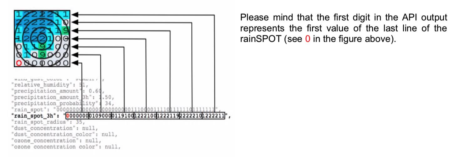
The indicated rainSPOT is the sum over the preceeding time period.
- This variable can be found in the following package: Basic
Snow
Snow is a special form of precipitation in the form of crystalline water ice, consisting of a multitude of snowflakes that fall from the clouds. As soon as snow settles on the surface, it is rapidly compressed by further snowflakes.
Snow Cover
It is the amount of accumulated snow (in mm) on the ground. This is a crude estimate and cannot be used to e.g. indicate how much snow is available in a particular ski resort.
The indicated snow cover applies to the point in time that is specified.
- This variable can be found in the following package: PV Pro
Snowfall Amount
Snow fall accumulates on the surface and can reach deposits of up to several meters in certain areas. Snowfall amount expresses the height of snow cover in centimetres (cm). As a rule of thumb, 10cm of fresh snowfall corresponds to 1cm of water.
The indicated snowfall amount is the sum over the preceeding time period.
- This variable is only available with Dataset API
Predictability
Predictability is the estimated certainty of our forecast. It considers uncertainties in pressure, precipitation, temperature, clouds, wind as well as climate inconsistencies. Predictability is expressed as percentage from 0% (worst) to 100% (perfect). Predictability is also subdivided into 5 classes: very low, low, medium, high and very high.
The indicated predictability applies to the point in time that is specified.
- This variable can be found in the following packages: Basic, Web Colors, Trend and Trend Pro
Pressure
Sea Level Pressure
It is the atmospheric pressure at sea level. For locations which are not at sea level, the pressure is corrected to represent pressure at sea level. Sea level pressure is expressed in hectopascal (hPa).
The indicated sea level pressure applies to the point in time that is specified.
- This variable can be found in the following packages: Basic, Trend, Trend Pro, Seasonal Anomalies Forecast and the History API
Radiation
Longwave Radiation / Heat Flux
Latent Heat Flux
Latent heat flux is the same than evapotranspiration- the sum of evaporation (soils, lakes, seas) and transpiration (plants). But it is expressed in watt per square meter (W/m).
The indicated latent heat flux is the average over the preceeding time period.
- This variable is only available with Dataset API
Sensible Heat Flux
Energy flux from the surface that is warming the air temperature. Sensible heat flux is expressed in watt per square meter (W/m ).
The indicated sensible heat flux is the average over the preceeding time period.
- This variable can be found in the following package: Agro
Solar Radiation
The indicated radiation is the average over the preceeding time period.
GHI (Shortwave Radiation)
Solar radiation is defined as the amount of total short-wave radiation energy reaching the horizontal Earth surface. Technically, it is also referred to as GHI (Global Horizontal Irradiance). The GHI can be split up into 3 components: diffuse, direct and reflected radiation. All radiation variables are measured in watt per square meter (W/m ) or joules per square centimetre (J/cm ).
The indicated GHI is the average over the preceeding time period.
- This variable can be found in the following packages: Solar, Solar Ensemble, Multimodel, Ensemble, Trend, Trend Pro and the History API
GNI (Global Normal Irradiance)
Global Normal Irradiance is the global irradiation on surfaces perpendicular to the sun rays (tracking the sun) and is expressed in watt per square meter (W/m ) or joules per square centimetre (J/cm).
The indicated GNI is the average over the preceeding time period.
- This variable can be found in the following package: Solar and the History API
GTI (Global Tilted Irradiation)
Global Tilted Irradiation is the global irradiance on a defined surface inclination, which is usually a PV module. All PV system simulations are based on the irradiation on the module plane. It is measured in watt per square meter (W/m ) or joules per square centimetre (J/cm ).
The indicated GTI is the average over the preceeding time period.
- This variable can be found in the following package: PV Pro
DIR (Direct Horizontal Irradiance)
The Direct Horizontal Irradiance is the directional share of the shortwave radiation(GHI). Direct radiation is coming from sun direction and therefore is also called circumsolar radiation. In cloudy sky condition, the direct radiation share is equal to 0. It is measured in watt per square meter (W/m) or joules per square centimetre (J/cm).
The indicated DIR is the average over the preceeding time period.
- This variable can be found in the following package: Solar and the History API
DNI (Direct Normal Irradiance)
Direct Normal Irradiance is the direct irradiance on surfaces perpendicular to the sun rays (tracking the sun). Of interest mainly for solar thermal and concentrated photovoltaic power generation. It is measured in watt per square meter (W/m ) or joules per square centimetre (J/cm).
The indicated is the average over the preceeding time period.
- This variable can be found in the following package: Solar and the History API
DIF (Diffuse Horizontal Irradiance)
Complementary to DIR (Direct Horizontal Irradiance) there is also Diffuse Horizontal Irradiance, which is defined as the scattered radiation or skylight. The diffuse share is very much depending on the sun height and on the clearness of the atmosphere. It is modelled according to Reindl and is expressed in watt per square meter (W/m) or joules per square centimetre (J/cm).
The indicated DIF is the average over the preceeding time period.
- This variable can be found in the following package: Solar and the History API
Clear Sky Solar Radiation
Clear sky solar radiation refers to the amount of solar energy that reaches the Earth's surface without being significantly affected by clouds, aerosols, or other atmospheric obstructions. It represents the theoretical maximum solar radiation under ideal atmospheric conditions.
- This variable can be found in the following package: Solar and the Dataset API
Extraterrestrial Solar Radiation
Maximum radiation intensity reaching the top of the Earth atmosphere is the extraterrestrial solar constant of 1368 W/m (1321 to 1413 W/m depending on distance of the Earth to the sun). It is dynamically modelled depending on the sun angle and expressed in watt per square meter (W/m) or joules per square centimetre (J/cm).
The indicated radiation is the average over the preceeding time period.
- This variable can be found in the following packages: Solar, Trend, Trend Pro and the History API
Photosynthetic Active Radiation
Photosynthetic active radiation (PAR) is electromagnetic radiation in a special range of the light spectrum which is mainly used by phototrophic organisms in photosynthesis. It covers most of the range of radiation with a wavelength between 380 nm and 780 nm (which is visible to humans).
The indicated photosynthetic active radiation applies to the point in time that is specified.
- This variable is only available with Dataset API
Photosynthetic Photon Flux Density
Photosynthetically active photon flux density (PFD or PPFD) is the current density of photons in the photosynthetically active solar spectrum. It is usually given in µmol(photons)/(m²s) in the range of wavelengths from 400 to 700 nm.
The indicated photosynthetically active photon flux density applies to the point in time that is specified.
- This variable is only available with Dataset API
IAM (Incidence Angle Modifier)
The glass surface of a PV system reflects the incoming radiation depending on the inclination angle. The Incidence Angle Modifier describes the share of radiation that is available for power generation. It has no unit and the value is always between 0 and 1.
- This variable can be found in the following package: PV Pro
Module Temperature
The Module Temperature describes the temperature of the solar cell. It is influenced by the outside temperature, the irradiation and the wind speed and has significant effect on the Performance ratio (PR). It's unit is °C.
The indicated heat flux applies to the point in time that is specified.
- This variable can be found in the following package: PV Pro
Performance Ratio (PR)
The performance ratio describes the efficiency of a power plant and varies significantly within different weather conditions. It is depending on surface reflectance, module temperature, spectral sensitivity and snow coverage and is expressed in percent (%).
The indicated performance ratio applies to the point in time that is specified.
- This variable can be found in the following package: PV Pro
PV Power
Photovoltaic power generation is the generated electricity power output of a specific PV system. The system efficiency to convert GTI to power is modelled depending on surface reflectance, module temperature, spectral sensitivity and snow coverage. It is expressed in kilowatt (kW) or kilowatt per hour (kW/h).
The indicated PV power is the average over the preceeding time period.
- This variable can be found in the following packages: PV Pro, Single Variable Multimodel and the History API
Snow Cover
The snow cover describes the height of snow on a horizontal surface. Based on the snow height the PV power output is adjusted. It is expressed in millimetres (mm).
The indicated snow cover applies to the point in time that is specified
- This variable can be found in the following package: PV Pro
Sunshine Time
Sunshine time is the amount of minutes with expected sunshine. It is indicated as minutes or hours respectively.
The indicated sunshine time is the sum over the preceeding time period.
- This variable can be found in the following packages: Clouds, Trend Pro and the History API
Daylight Duration
Daylight duration is defined as the time between sunrise and sunset. It is dependent on the latitude and the time of the year. It is given in minutes per hour (min/h).
- This variable is only available with Dataset API
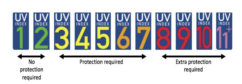
UV Index
The ultraviolet index (UV index) is an international standard measurement of the strengths of the ultraviolet radiation from the sun. The purpose is to help people to effectively protect themselves from UV light. The UV index value always refers to the highest possible value that can be achieved at midday. It is expressed in index numbers from 1 to 16. Note that values above 11 should be shown as 11+. This is illustrated in figure below
- This variable can be found in the following packages: Basic and Web Colors
Sea Variables
Sea Surface Temperature (SST)
Mean temperature of the ocean in the upper few meters. Note that water temperatures at the beach might be warmer than indicated by the SST (due to decreasing water depth). The SST is indicated in degrees Celsius (°C).
The indicated surface temperature applies to the point in time that is specified.
- This variable can be found in the following packages: Sea and Seasonal Anomalies Forecast
Peak- / Primary- / Swell- / Wind-Waves
Peak Wave: The highest wave in a set of waves or period of time, typically of interest to surfers.
Primary Wave: The dominant wave-type in a sea state, typically the largest and with the most energy.
Swell Wave: Long, smooth waves that have traveled far from their origin (thousands of kilometres), unaffected by current local winds. Long-period swells accumulate energy, travel faster, and can easily withstand local winds and currents, resulting in larger surf with regard to average wave height.
Wind Wave: Short, choppy waves created by local wind conditions, more irregular in shape and shorter-lived.
- These variables can be found in the following package: Sea, as well as in the WAM-series in the Dataset API.
Significant Wave Height (Swell-/Wind-Waves) [m]
Swell waves can be very large even if there is no local wind. The significant height of swell waves is the average of the highest 33% of the swell waves over a given time period.
The significant height of wind waves is the average height of the 33% highest waves generated by the local wind over a given time period. Wind waves are only generated if local winds are sufficiently strong.
The wave height is indicated in metres (m) and applies to a specified point in time. Wave height values are averaged numbers, so some individual waves can be much higher.
- These variables can be found in the following package: Sea, as well as in the WAM-series in the Dataset API.
Mean Wave Period (Swell-/Wind-Waves) [sec]
The mean period of ocean waves refers to the average time interval between successive wave crests (or troughs) passing a fixed point. The wave period influences wave energy and the impact on structures and shorelines. Typically, the mean period of ocean waves can range from a few seconds to around 20 seconds, depending on various factors including wind speed, fetch (the distance over which the wind blows), and the overall sea state. The following holds true as a general rule:
- Wind waves have shorter periods, generally between 1 to 10 seconds.
- Swell waves have longer periods, usually between 10 to 20 seconds.
The primary wave period describes either the period associated with the locally generated winds (in cases with strong local winds) or the dominant wave system (swell) that is generated elsewhere. Note that high energy waves produced with strong winds have lower frequencies (or longer periods) and that the peak wave period increases (wave frequency decreases) until it reaches equilibrium. The indicated mean period applies to the point in time that is specified.
The mean period is of major interest for waveriding/surfing, since it ultimately measures the quality of the upcoming surf session. The following table describes different wave periods:
| Wave Period [s] | Waveriding/Surfing Conditions |
|---|---|
| 1 - 5 | Local gusts of wind with bumpy and disordered wind waves, poor surfing conditions. |
| 6 - 8 | Regional and local gusts with average surfing conditions, offshore winds may improve surfing conditions. |
| 8 - 10 | Medium-distance swell-waves, above-average local surfing conditions. |
| 10 - 15 | A long period swell brings high-quality waves, great surfing conditions. |
| 15+ | The power of long-period groundswells is taking effect (energy of long-period waves extends down into the water and comes into contact with the ocean floor earlier than waves of shorter period), excellent surfing conditions. |
- These variables can be found in the following package: Sea, as well as in the WAM-series in the Dataset API.
Mean Wave Direction (Swell-/Wind-Waves) [°]
The direction of the wind wave is defined by the origin of the corresponding wind, using the same convention as for wind direction (degrees). The direction of swell waves indicates their pre-travel origin, also measured in degrees. The peak wave direction indicates the directional movement of the dominant wave system, i.e. the swell with the maximum energy. For locations with multiple swell systems, the peak wave direction refers to the direction of the swell with the highest energy. The indicated wave direction applies to the point in time that is specified.
- These variables can be found in the following package: Sea, as well as in the WAM-series in the Dataset API.
Soil variables
Soil Moisture
Soil moisture is the mean moisture of the uppermost 10 cm of soil. It is indicated as volumetric percentage. The volumetric soil moisture (m³/m³) indicates how much of m³ soil is water. It is the volumetric fraction of water: 0.3 m³/m³ are 30 vol. %. Typically values are in between 0.15 and 0.45. Note that soil moisture will mainly show larger seasonal variations but not give significant signals on a daily or weekly basis.
The indicated soil moisture applies to the point in time that is specified.
- This variable can be found in the following package: Agro and the History API
Soil Temperature
Soil temperature is the average temperature of the uppermost 10 cm of soil.
The indicated soil temperature applies to the point in time that is specified.
- This variable can be found in the following package: Agro and the History API
Storm Prediction/ Convective Weather Variables
Air Density
Air density decreases rapidly with altitude and also with increasing temperature and humidity.Unit of measurement is kilogram per cubic metre (kg/).
The indicated density applies to the point in time that is specified.
- This variable can be found in the following packages: Wind and Sigma Level
(Planetary) Boundary Layer Height
Boundary layer height is expressed in meters (m). It is the height up to which air and pollutants (originating from the surface) are mixed up to. If the boundary layer height remains low during the entire day and over several days, than air quality can significantly decrease. A typically daily course is seen in the boundary layer height with maximum values in the afternoon and minimal values during the night.
The boundary layer height also might be called planetary boundary layer height (PBL-Height).
The indicated boundary layer height applies to the point in time that is specified.
- This variable can be found in the following package: Air
CAPE
Convective available potential energy (CAPE) is the available amount of energy for convection. The higher the value, the greater the potential for severe weather. It is expressed in joules per kilogram (J/kg). Observed values in thunderstorm environments often may exceed 1000 joules per kilogram (J/kg) and in extreme cases may exceed 5000 J/kg.
- CAPE < 1000J/kg = weak instability
- CAPE > 1000J/kg = moderate instability
- CAPE > 2500J/kg = strong instability
The indicated CAPE applies to the point in time that is specified.
Lifted Index (LI)
The lifted index is a measure of atmospheric instability. The temperature value of the ground is computed and compared with the actual temperature at a specific pressure height. The difference between both values is the lifted index. The air is stable for positive index numbers and unstable for negative index numbers. The more negative, the more unstable the air is, and the stronger the updrafts are likely to be with any developing thunderstorms. However there are no "magic numbers" or threshold LI values below which severe weather becomes imminent but some people use the following rule of thumb:
- LI 6 or greater = very stable conditions
- LI between 1 and 6 = stable conditions, thunderstorms not likely
- LI between 0 and -2 = slightly unstable, thunderstorms possible with lifting mechanism (e.g. cold front, daytime heating etc.)
- LI between -2 and -6 = unstable, thunderstorms likely, some severe with lifting mechanism
- Li less than -6 = very unstable, severe thunderstorms likely with lifting mechanism
The indicated lifted Index applies to the point in time that is specified.
Helicity
Identifies the potential for helical flow (e.g. flow which follows the pattern of a corkscrew) to evolve. It can be useful to identify thunderstorm types. It is expressed in meters square per second squared (m /s ). Rule of thumb:
- 0-50 m/s = low possibility for storms, thunderstorms and tornadoes
- 100 m/s = strong thunderstorms
- 150- 200 m/s = tornados likely
Note however that this should not be used as automated tool to forecast tornadoes, it is rather one factor an experienced meteorologist considers together with many others when issuing tornado warnings.
The indicated helicity applies to the point in time that is specified.
- This variable can be found in the following package: Air
Convective Inhibition (CIN)
A measure of the unlikelihood of thunderstorm development. It represents the amount of energy which an air parcel needs, to reach the level of free convection. Low level air parcel ascent is often inhibited by stable layers near the surface. If natural processes fail to destabilize the lower levels, an input of energy from forced lift (a front, an upper level shortwave, etc.) will be required to move the negatively buoyant air parcels to the point where they will rise freely. Since CIN is proportional to the amount of kinetic energy that a parcel loses to buoyancy while it is colder than the surrounding environment, it contributes to the downward momentum. Convective inhibition is expresses in joules per kilogram (J/kg). The presence of CIN doesn't preclude thunderstorm development as long as it isn't too high. In fact, a moderate amount of CIN in the morning hours is actually favourable to the development of heavy afternoon thunderstorms in the presence of a large amount of CAPE. High CAPE and low CIN morning environments tend to cloud up very quickly after a small amount of surface heating is introduced. Watch for the CIN to go to zero in the afternoon on high CAPE days. This is warning flag that afternoon convection is likely (at least from the point of view of the model). Rule of thumb:
- CIN < 50J/kg = weak cup that can e easily broken by surface heating
- CIN between 50 and 200J/kg = moderate cap that can be broken by strong heating/synoptic scale forcing
- CIN > 200J/kg = strong cap impedes thunderstorm development.
The indicated CIN applies to the point in time that is specified.
- This variable can be found in the following package: Air
Temperature
Air Temperature
Air temperature is calculated for 2 meters above the ground at any given location and altitude. Temperature is expressed in degrees Celsius (°C) and degrees Fahrenheit (°F).
The indicated air temperature applies to the point in time that is specified.
- This variable can be found in the following packages: Basic, Current, Web Colors, Sigma Level, Profile Series, Multimodel, Single Variable Multimodel, Ensemble, Trend, Trend Pro, Seasonal Anomalies Forecast, Modelclimate and the History API
Felt Temperature
Felt temperature is the perceived temperature that people experience. It considers the cooling effect of wind (wind chill) as well as heating effects caused by relative humidity, radiation and low wind speeds. It is expressed in degrees Celsius (°C) and degrees Fahrenheit (°F).
The indicated felt temperature applies to the point in time that is specified.
- This variable can be found in the following packages: Basic and Web Colors
Skin / Surface Temperature
Skin or surface temperature is also called radiative temperature and is a measure of the temperature of the surface. It is expressed in degrees Celsius (°C) and degrees Fahrenheit (°F).
The indicated skin/ surface temperature applies to the point in time that is specified.
- This variable can be found in the following packages: Agro, Ensemble, Trend Pro and the History API
Wet Bulb Temperature
Wet bulb temperature is the temperature measured by a thermometer covered with a water-soaked cloth over which air circulates. The wet bulb temperature is the lowest temperature that can be achieved by direct evaporative cooling. Because of evaporative cooling, the wet bulb temperature is lower than the air temperature, depending on the relative humidity. At 100% RH, the wet bulb temperature is equal to the air temperature.
The indicated wet bulb temperature applies to the point in time that is specified.
- This variable can be found in the following package: Agro and the History API
Temperature Spread
Temperature spread indicates the uncertainty in the forecast as computed by the ensemble prediction. It is defined as one standard deviation of the computed variation and is expressed in degrees Celsius (°C) and degrees Fahrenheit (°F).
- This variable can be found in the following packages: Multimodel, Ensemble and Trend
Wind
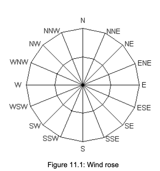
Wind Direction
It is the direction from which the wind blows (e.g. north wind comes from the north and blows to the South corresponding to a direction of 0 degrees). It is expressed in degree (°), 2 characters and 3 characters for 10 or 80 meters above ground. The following table illustrates the correspondence of wind direction to degrees and the wind rose gives an overview over cardinal wind directions:
| Cardinal Direction | Degree Direction |
|---|---|
| N | 348.75 – 11.25 (0/ 360) |
| NNE | 11.25 - 33.75 |
| NE | 33.75 - 56.25 |
| ENE | 56.25 - 78.75 |
| E | 78.75 - 101.25 |
| ESE | 101.25 - 123.75 |
| SE | 123.75 - 146.25 |
| SSE | 146.25 - 168.75 |
| S | 168.75 – 191.25 |
| SSW | 191.25 - 213.75 |
| SW | 213.75 - 236.25 |
| WSW | 236.25 - 258.75 |
| W | 258.75 – 281.25 |
| WNW | 281.25 - 303.75 |
| NW | 303.75 - 326.25 |
| NNW | 326.25 - 348.75 |
Used presentations of wind directions:
-
Arrows: The arrowhead points to the direction to which the wind blows:
- → West wind- comes from the West and blows to the East
- ← East wind-comes from the East and blows to the West
- ↓ North wind- comes from the North and blows to the South
- ↑ South wind- comes from the South and blows to the North
-
Wind barbs: The wind barb shows the wind direction along with wind speed. The part of the barb with the attached feather(s) points in the direction from which the wind comes.
Figure: Wind barbs for North-West wind

- Degrees:
0°/ 360°(North): Wind blows from the North to the South (↓)
90° (East): Wind blows from the East to the West (←)
180°(South): Wind blows from the South to the North (↑)
270°(West): Wind blows from the West to the East (→)
- Characters
- 1 character: North (N), West (W), South (S), East (E) → 90° distance
- 2 character: N, NW, SW, W, SE, E, NE, E → 45° distance
- 3 character: N, NNE, NE, ENE, E, ESE, SE, S etc. → 22.5° distance
The indicated wind direction is the average over the preceeding time period.
- This variable can be found in the following packages: Basic, Wind, Sigma Level, Profile Series, Multimodel, Ensemble, Trend, Trend Pro, Climate Wind Rose and the History API
Wind Gust
Wind gusts indicate how turbulent the wind is. It is the speed that can be expected for short periods of time, which can be much higher than the wind speed, which is an hourly mean wind speed. This value can vary enormously. If you are not interested in the turbulence information you might slightly modify the gust wind for displaying it to your users by making sure the gust winds are always larger or equal to the mean wind speed, to avoid confusion why the gust should be smaller than the mean wind speed.
Gust wind is expressed in meters per second (m/s), kilometres per hour (km/h), miles per hour (mph), knots (kn) and beaufort (bf) for 10 or 80 meters. As gust wind are turbulent it is not possible to predict a direction of the gusts as it varies randomly.
The indicated wind gust applies to the point in time that is specified.
- This variable can be found in the following packages: Wind, Ensemble, Trend Pro and the History API
Wind Speed
Wind speed is the rate at which air is moving horizontally. meteoblue expresses wind speed in meter per second (m/s), kilometres per hour (km/h), miles per hour (mph), knots (kn) and beaufort (bf). Wind speed is expressed as an hourly mean value. Wind is very turbulent and thus the actual wind speed can be much higher than indicated by the mean wind, but only for short time periods. This short periods of high wind speed are called gusts. Typical gusts speed which can be expected are indicated by the variable gust wind. Unless otherwise marked in the variable name it is valid for 10 m above ground. Windspeed 80m would be valid at 80 m above ground.
The indicated wind speed is the average over the preceeding time period.
- This variable can be found in the following packages: Basic, Current, Wind, Wind 80m Ensemble, Sigma Level, Profile Series, Multimodel, Single Variable Multimodel, Ensemble, Trend, Trend Pro, Seasonal Anomalies Forecast, Modelclimate, Climate Wind Rose and the History API
Wind Speed Spread
Wind speed spread indicates the uncertainty in the forecast as computed by the ensemble prediction. It is defined as one standard deviation of the computed variation and indicated in meters per second (m/s).
The indicated wind speed spread is the average over the preceeding time period.
- This variable can be found in the following packages: Multimodel, Trend and Trend Pro